ArcGIS Geostatistical Analyst: The Science of Interpolation and Prediction from Sparse Data

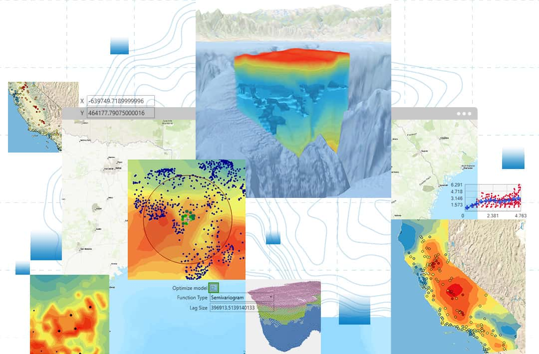
In many fields, we can only collect data at a limited number of locations — for example, measuring air quality at a few monitoring stations, taking soil samples at a few points in a field, or drilling exploratory boreholes at a few locations in a mine. So how can we create a continuous prediction map for the entire area from those discrete data points? ArcGIS Geostatistical Analyst is the answer. It is a specialized extension for ArcGIS Pro that provides a scientific toolset to analyze, interpolate and map spatial phenomena from point datasets.

In essence, Geostatistical Analyst does not simply “connect” data points together. It uses sophisticated statistical methods based on the principle that “everything is related to everything else, but near things are more related than distant things” (the First Law of Geography). This allows it to produce prediction surfaces that carry not only estimated values but also an uncertainty map, telling you how reliable the prediction is at each location.

Technical Capability Groups and Practical Applications

Working with Geostatistical Analyst typically follows a rigorous scientific cycle, from data exploration to model building and evaluation.

1. Exploratory Spatial Data Analysis (ESDA)

Before interpolating, you need to “understand” your data. This group of tools lets you visualize and detect patterns, trends and outliers.

• Technical capabilities:
  • Histogram: Checks the distribution of data values (for example: whether they follow a normal distribution).
  • Trend Analysis: Determines whether there is an overall trend in the data in a particular direction (for example: temperature tends to increase from north to south).
  • Semivariogram/Covariance Cloud: The core tool for examining spatial autocorrelation. It plots how different pairs of data points are, based on the distance between them.
  • Voronoi Map: Partitions the space around data points to identify neighborhood areas.
• Practical applications:
  • Environment: Before mapping pollution, an analyst uses ESDA to see whether pollutant concentrations tend to rise near industrial zones.
  • Agriculture: A soil scientist uses a Histogram to check whether the pH of soil samples follows a normal distribution, an important assumption for some interpolation methods.
  • Geology: Trend analysis is used to determine the main direction of an underground mineral seam.

2. Spatial Modeling and Interpolation

This is the heart of Geostatistical Analyst, offering many methods for creating continuous prediction surfaces. These methods fall into two main groups:

• A. Deterministic Methods:
  • Technical capabilities: These methods create surfaces based on deterministic mathematical formulas, relying mainly on similarity or distance.
    • Inverse Distance Weighted (IDW): Predicts the value at a location based on the values of neighboring points, assuming that closer points have greater influence.
    • Radial Basis Functions: An exact interpolation method that produces a smooth surface passing through all input data points.
• B. Geostatistical Methods:
  • Technical capabilities: These methods are based on both statistics and mathematics, producing not only a prediction surface but also surfaces that measure error and uncertainty.
    • Kriging: A family of interpolation methods regarded as the “gold standard”. Kriging analyzes the spatial relationships in the data (through the semivariogram) to produce an optimal prediction surface. Common forms include:
      • Ordinary Kriging: The most common form, assuming the mean is constant but unknown.
      • Universal Kriging: Used when the data has a clear trend.
      • Indicator Kriging: Predicts the probability that a value will exceed a given threshold (for example: the probability that a pollutant concentration exceeds the safe limit).
    • Cokriging: An advanced form that uses information from one or more related secondary variables to improve prediction accuracy.
• Practical applications:
  • Meteorology: Use Ordinary Kriging to create a detailed rainfall map for a province from rain gauge station data.
  • Public health: Use Indicator Kriging to create a map of the “probability of lead exposure” in children exceeding the permitted threshold, helping health agencies delineate areas that need urgent intervention.
  • Mining: Geological engineers use Kriging to estimate gold grade in a mining area, while also producing an error map to identify where additional exploratory boreholes should be drilled to reduce uncertainty.
  • Precision agriculture: Use Cokriging to create a soil nutrient map (for example: nitrogen concentration), adding elevation data (an easily collected secondary variable) to improve accuracy.

3. Model Diagnostics and Validation

After creating a surface, how do you know how good it is? This group of tools helps you assess the accuracy of the interpolation model.

• Technical capabilities:
  • Cross-validation: An automated technique in which the system temporarily removes each data point in turn, then uses the remaining points to predict the value at the removed point. By comparing predicted and actual values, it provides an objective measure of model accuracy.
  • Validation: If you have a separate dataset for testing, this tool lets you compare the model’s predicted values against that validation dataset.
• Practical applications:
  • Environment: A scientist compares several different Kriging models (with different parameters) using the cross-validation tool. They choose the model with the lowest mean prediction error to produce the final pollution map.
  • Risk management: An insurance company uses validation results to assess the reliability of a flood risk prediction model before applying it to calculate premiums.

Conclusion

ArcGIS Geostatistical Analyst is not just a tool for producing attractive interpolation maps. It is a complete scientific toolset that brings statistical rigor to spatial prediction. By allowing users not only to produce predictions but also to understand and quantify their uncertainty, it helps scientists, planners and managers make data-driven decisions with greater confidence and accountability.